Area payments are a key instrument of the European Union’s Common Agricultural Policy. However, their effectiveness as a tool for supporting farmers’ incomes is weakened by the phenomenon of capitalisation. The aim of this study is to identify the mechanism by which area payments stimulate inputs of agriculture production factors and to examine how subsidies granted in the form of area payments are transformed into remuneration for production factors. The research methodology used includes economic modelling and marginal analysis. It is demonstrated that area payments change the allocation of resources compared to the allocation driven by the market mechanism (resulting in a greater engagement of production factors in agricultural production than would be the case in the absence these subsidies) and also affect the level and structure of the remuneration for production factors in agriculture. A theoretical decomposition of the remuneration of production factors into income from non-land production factors and land rent has been carried out.
Keywords:
Agricultural financial support, Area payments, Land rent, Lease rent, Payments’ capitalization
Sadłowski: Model of the Impact of Area Payments on the Engagement and Remuneration of Production
Factors in Agriculture
1. INTRODUCTION
EU agricultural subsidy instruments under the Common Agricultural Policy (CAP) have
evolved from supporting agricultural production to supporting farmers’ incomes and
stimulating the supply of public goods (; ; ; ; ). Area payments introduced several decades ago, remain a key instrument of CAP’s
Pillar I. However, many agricultural economists argue that, despite reforms, these
payments are still insufficiently effective in encouraging farmers to provide public
goods and are inadequately tailored to the environmental and social dimensions of
sustainable development (; ; ; ).
Direct payments, including area payments that dominate in terms of the EU agricultural
budget expenditures, are intended by lawmakers to support farmers’ incomes and stimulate
the production of public goods while minimizing unintended side effects. Unintended
side effects of area payments include distorting the volume and structure of the agricultural
output shaped by the market mechanism and perpetuating production systems or agricultural
practices that have a significant negative impact on the environment (; ; ; ; ; ; ; ; ). Area payments also influence farms’ demand for production factors, including agricultural
land (; ; ).
The purpose of this study is to identify the mechanism by which area payments stimulate
the input of production factors in agriculture and the mechanism through which subsidies
in the form of area payments are transformed into remuneration for production factors.
The structure of the article is as follows. After the introductory section, which
briefly presents the research topic, objective, and structure of the study, a review
of literature on the phenomenon of “capturing” area payments by non-farming entities
or individuals who own agricultural land is provided (this is referred to in the literature
as the capitalization of area payments into lease rents or agricultural land prices).
The next section is devoted to the description of the methodology of the theoretical
research conducted. In the section titled “Results and Discussion”, the essence of
the proposed model of the impact of area payments on the level of utilization and
remuneration of production factors in agriculture is presented, along with definitions
of indicators derived from this model using analytical tools, namely (i) the degree
of agricultural activity subsidization, (ii) the level of state co-financing of land
rent, and (iii) the conversion of area payments into land rent. In the summary section,
conclusions are drawn, along with the advantages and limitations of the presented
model.
2. LITERATURE REVIEW
The phenomenon of area payment capitalization has been addressed as a key research
problem or one of the aspects of studies by many agricultural economists (Table 1). Among the relatively numerous publications in this field, many are empirical studies
based on data of varying temporal and spatial scope. Additionally, different research
methods are often employed. This section summarizes the main findings of studies related
to instruments used under the CAP.
Table 1General characteristics of the major studies on capitalization of payments
Reference to publication
Type of studies
Spatial scope
Subject scope
theoretical
EU Member States applying the Single Payment Scheme (SPS)
land rents land prices
empirical
Northern Ireland
land rents
review
EU
land rents land prices
empirical
EU Member States applying the Single Area Payment Scheme (SAPS)
land rents
empirical
Bavaria (Germany)
land rents
review
EU
land prices
empirical
EU Member States applying the SPS
land prices
empirical
Wielkopolskie Voivodeship (Poland)
land prices
empirical
EU
land prices
empirical
Ireland
land rents
empirical
Bavaria (Germany)
land rents
empirical
EU
land prices
review
Germany
land rents land prices
theoretical
EU
land rents
empirical
West German federal states
land rents
review
EU
land prices
empirical
EU Member States applying the SPS
land prices
empirical
Bavaria (Germany)
land rents
review
EU
land prices
empirical
EU
land rents land prices
The CAP reforms, including the reform that decoupled payments from production, provided
an impetus for research on the impact of changes on the intensity of capitalization.
, summarizing the results of their research on the impact of the Fischler CAP reform
on agricultural land prices, found that a reduction of payments by 50 EUR/ha would
decrease land sales prices by 445 EUR/ha before and by 984 EUR/ha after the reform.
also focused on the impact of the 2013 CAP reform on the capitalization of payments.
They concluded that on average in the EU, the non-farming landowners’ policy gains
are 27% of the total decoupled payments in the post-reform period, compared to 18%
in the pre-reform period. found that the impact of direct payments on rental values depends on the type of
payment (coupled or decoupled payments) and the nature of the production of the associated
agricultural commodity. According to , the introduction of decoupled payments increased the capitalization rate, although
the extent of this increment hinges on the implementation scheme adopted by the EU
member state. noted that in Ireland coupled direct payments were highly capitalized into land rents
(67–90 cents per 1 EUR of subsidies). emphasize that with the decoupling of direct payments from production, given the
overall high share of rents in Germany, an increasing share of payments indirectly
goes to landowners, with the size of this transfer varying considerably depending
on the period, region and share of tenancy.
Numerous studies were aimed at identifying the extent to which individual systems
and models of direct payments applied under the CAP contribute to the intensification
of the capitalization phenomenon. According to , the capitalization outcome crucially depends on the proportion of eligible agricultural
areas to payment entitlements and which model of SPS (historical, regional, or hybrid)
has been implemented. estimated a 6–10% SPS capitalization rate. They found that on average in the EU,
the nonfarming landowners’ gains from the SPS are 4%, however, there is a large variation
in the capitalization rate for different SPS levels and between different member states
(3–94%). find that between 28 and 52 cents per 1 EUR of additional subsidy capitalize into
land prices in EU member states that adopted the hybrid and the regional model, respectively,
whereas in EU member states that adopted the historical model subsidies do not capitalize
in farmland prices. The specificity of SAPS applied in most new EU Member States was
also addressed. According to , SAPS contributes to land value mainly in the peripheral areas and payments for public
goods under SAPS decapitalize the value of land, because they do not compensate for
the opportunity costs related to alternative ways of deriving rent from the land.
found that land rents capture 19 cents of the marginal SAPS, and around 10% of the
SAPS benefit nonfarming landowners through higher farmland rental prices.
The capitalization phenomenon has been well recognized and measured in Bavaria. , based on research conducted using data for this German federal state relating to
the year 2005, found that decoupled direct payments are capitalized into rental prices
to a larger degree than the coupled payments of the time before the 2003 CAP reform.
investigated the impact of the gradual harmonization of direct payments on the level
of rents, concluding that strong capitalization effects increased substantially in
the period since 2010 when Germany began harmonizing payments: on average, the marginal
effect on rental rates of an additional 1 EUR paid under SPS is 37 cents, growing
to 53 cents as harmonization develops. , also based on data for Bavaria, find that on average 30% of direct payments are
capitalized into land rental prices, and the capitalization ratio varies considerably
across regions.
generalized the results of earlier studies, finding that a 10% reduction in agricultural
support would reduce land prices by 3–5%. Later research results of indicate that 10–12% of the overall CAP payments were leaked to non-farming landowners
in 2016. However, there is a sizeable variation in the non-farming landowners’ gains
across EU member states, ranging from 2% to 37%. noted that the effect of direct payments on land rental prices depends on the competitiveness
of the market; under certain conditions, the transfer of subsidy may be total, but
in practice, it is usually relatively low.
The issue of payments’ capitalization was also addressed about a specific type of
land use, namely permanent grassland. found that landlords of grassland in West German federal states have benefited strongly
from the decoupling of direct payments. At the end of the observation period, covering
the years 2001–2013, after regional standardization of the payments, the estimates
show marginal capitalization rates of 87–94 cents per additional 1 EUR, which means
almost complete capitalization of the subsidies into the rental price for grassland.
concluded that agricultural support policy instruments contribute to increasing the
rental price of farmland and that the extent of this increase closely depends on the
supply price elasticity of farmland relative to those of other factors/inputs on the
one hand and the range of the possibilities of factor/input substitution in agricultural
production on the other hand. In addition, they stated that land prices are more responsive
to government-based returns than to market-based returns. These conclusions have not
lost their significance, however, a more recent summary of research in this area is
the work by . Taking into account the results of theoretical analyses and empirical research on
the capitalization of agricultural subsidies into land prices, they concluded that
the theoretical literature predicts that agricultural subsidies are capitalized into
land prices when land supply is inelastic and land markets function well, and the
capitalization rate significantly depends on the shape of subsidies, level of development
of local land-market institutions, and spatial effects. Simultaneously, most empirical
studies have shown that agricultural subsidies are only partially capitalized into
land prices, and decoupled payments and land-based subsidies exhibit higher capitalization
than coupled payments and nonland-based subsidies, respectively.
Capitalization of support in lease rents and land prices can be considered the main
cause of the inefficiency of financial transfers, which are intended to improve farmers’
income situations (; ). This should be viewed as an undesirable side effect of the direct support system,
which increases the wealth of agricultural landowners and creates barriers to entry
into the sector (; ).
3. MATERIALS AND METHODS
The theory explaining the mechanism of the impact of area payments on the production
sphere (the level of engagement of production factors) and the distribution sphere
(remuneration of production factors) was developed using economic modelling. In the
model, land remuneration is interpreted, in line with Ricardo’s land rent theory (), as a residual amount remaining after the costs of other production factors have
been covered.
The research method employed is marginal analysis (i.e., analysis of marginal changes
in economic variables). In the model, marginal revenue is not defined as the increase
in total revenue due to an increase in production (and simultaneously sales) by one
unit, but rather as the increase in total revenue resulting from the use of an additional
unit of land. Similarly, marginal cost is understood as the ratio of the increase
in total cost (non-land production inputs) to the increase in land input by one unit.
The model adopts the perspective of a farm that is a “price taker” – both in the agricultural
product market and in the market for production factors. This means that the individual
decisions of a single farm regarding production volume or resource engagement do not
affect their market prices.
The structure of the model is dual. The baseline scenario, in which no area payments
are applied (zero variant), is compared with a scenario where this form of government
intervention in agriculture is applied (alternative variant). This allows for the
identification of the economic effects of the intervention. Understanding the mechanism
of converting area payments into the remuneration of production factors provided a
framework for describing and measuring the phenomenon of “capturing” support paid
to farmers by landowners.
The developed model is a tool for analysing the behaviour of a farm as an economic
entity, making it a microeconomic model. It allows for determining the optimal level
of land resource utilization in the farm, thus making it an optimization model. At
the same time, it is an equilibrium model, as it indicates the operation of an automatic
mechanism by which the farm reaches a state of equilibrium, where there are no further
incentives for change.
The impact of financial incentives in the form of area payments on the decisions of
a single farm was modelled. Since this instrument affects the entire community of
farms in the same way, it causes typical adjustments of these farms in the same direction
in relation to the size of inputs. This makes it possible to generalize the findings
made at the microeconomic level to the national level. This is because equilibrium
across the entire agricultural sector corresponds to individual (farm) equilibrium.
The essence of the model is presented using graphical methods of visualizing relationships
(charts) accompanied by descriptive methods. The analysis is theoretical in nature
and therefore not based on specific figures or statistics relating to the general
population or a part (subset) of it. As no empirical data were used directly, an indication
of the temporal and spatial scope of the study is not applicable here. Although the
inspiration for the considerations was the area payments applied in the EU under the
CAP, the proposed model is universal. This nature of the model made it possible to
formulate conclusions of general applicability, abstracting from time and place. The
analysis carried out should be considered static, as it focuses on comparing two states
(without and with area payments), using equilibrium modelling.
4. RESULTS AND DISCUSSION
4.1. Area Payments and Land Input
4.1.1. Optimal Level of Land Engagement
Area payments are characterized by linking the amount of granted support to the area
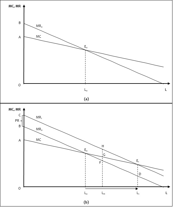
of agricultural land used. Figure 1(a) illustrates the zero variant, i.e., a situation where this instrument is not applied.
On the horizontal axis of the coordinate system, the amount of land input (in surface
units, e.g., hectares) is plotted. Moving rightward along this axis reflects decreasing
agricultural suitability of the land, as the most fertile and easily accessible plots
are engaged in production first. Meanwhile, the vertical axis represents the level
of a given economic variable, expressed in monetary units per unit of land input (homogeneous,
single agricultural plot). The economic variables included in the chart in Figure 1(a) are marginal production cost, covering inputs of non-land production factors (i.e.,
labour and capital in the classical sense), and marginal revenue from the sale of
agricultural produce. In the chart shown in Figure 1(b), the marginal revenue function graph in position MR1 – besides revenue from the sale of agricultural products – also includes revenue
from area payments.
The graph of the marginal cost (MC) function, understood as the increase in total
costs (i.e. non-land production inputs) resulting from an increase in land input by
one unit, is a declining line because the less fertile the land, the lower the amount
of labour and capital required to maximize economic result (). The graph of the marginal revenue function (MR0), understood as the increase in total revenue from an increase in land utilization
by one unit, is also a declining line. The negative slope of this line results from
the fact that the most productive lands, generating the highest revenue from the sale
of agricultural produce at given inputs, are engaged in production first. As less
fertile and more peripherally located lands are engaged in the production process
(moving rightward along the horizontal axis), the marginal revenue from each subsequent
unit of land decreases.
The relative position of the graphs of the marginal cost and marginal revenue functions
in Figure 1 is a consequence of the assumption that there are lands on which agricultural production
is profitable even without area support (MR0 runs above MC; these are lands located to the left of L0, i.e. those with the greatest agricultural usefulness), and at the same time there
are lands on which agricultural production would result in a loss (MR0 runs below MC; these are lands located to the right of the L0 point).
The area under the marginal cost (MC) curve represents total costs (TC), while the
area under the marginal revenue (MR0) curve represents total revenue (TR). The optimal level of land resource utilization
in agricultural production is determined by the first coordinate of the intersection
point of the MC function with the MR0 function (E0), i.e., L0. At this level of land input, the economic result, understood as the surplus of total
revenue over cost, is maximized, so the input of production factors other than land
is also optimal.
Figure 1Level of land resource utilization in the variant without area payments (a) and with
area payments (b)
In contrast, Figure 1(b) illustrates a situation where agricultural activities are subsidized through the
provision of financial support to farms proportional to the area of agricultural land
used. In this case, production factors engaged in the production process are remunerated
not only by the market (in the form of revenues from the sale of agricultural produce)
but also by the state (in the form of area payments).
The rates of direct payments can be counted among the parameters of the economic calculation,
which constitute the systemic conditions of management in agriculture. Farmers are
forced to take payment rates into account in their economic decisions, although this
is not enforced administratively, but by the threat of obtaining a worse economic
result ().
The area payment rate is uniform (not differentiated regionally or by land quality),
so the introduction of this instrument can be graphically represented by a parallel
upward shift of the MR0 revenue function graph – by a segment |BC|, the length of which corresponds to the
area payment rate PR – into position MR1. As a result, the new equilibrium point for the farm will be point E1, corresponding to a higher level of land input (L1>L0). Thus, lands that were previously not used for agricultural production (in the absence
of area support) will be engaged in agricultural production. The length of the |L0L1| segment reflects the size of the additional land area (i.e., land engaged in production
due to the introduction of area payments).
Thus, area support provides an incentive for farms to increase land input, leading
to an increase in the total area of agricultural land used in the country. However,
if resource management is to be rational, there is no justification for increasing
this area for reasons other than improved market conditions in agriculture.
4.1.2. Effects of Price Changes
The model allows for the consideration of price changes (in any direction) in both
the markets for production factors and agricultural products. An increase/decrease
in the prices of agricultural inputs or wages would result in an upward/downward shift
of the marginal cost (MC) function graph. Meanwhile, an increase/decrease in the prices
of agricultural products would be reflected in an upward/downward shift of the marginal
revenue (MR) function graph.
4.1.3. Impact of Agricultural Tax
The presented model can also incorporate the impact of agricultural tax on the analysed
variables. Given that the amount of agricultural tax decreases with the declining
agricultural suitability of land, its effect can be represented by a non-parallel
upward shift of the marginal cost function graph, proportional to the tax amount,
such that the new function (MC1) converges with the original function (MC0) as it moves rightward along the horizontal axis. However, in the first quadrant
of the coordinate system (where the analysis is conducted, as it corresponds to the
values of the examined variables that make economic sense), there would be no intersection
of these function graphs.
4.2. Area Payments and Remuneration of Production Factors
4.2.1. Land Rent as a Residual Amount
The remuneration for land, as a resource engaged in the production process, is a residual
amount representing the surplus of revenues from the sale of agricultural produce
(in the variant with area payments – increased by the revenues from these payments)
over the production costs, which include inputs of non-land production factors. This
is equivalent to economic profit. This conclusion recalls the Physiocratic thesis
that land is the only surplus-generating production factor ().
In the variant without area payments, as shown in Figure 1(a), the total remuneration for land at the farm’s equilibrium point (E0) is represented by the area of triangle AE0B. Meanwhile, the amount of land rent per unit of land area (homogeneous in terms
of agricultural suitability) is symbolized by the vertical distance between the marginal
cost (MC) function graph and the marginal revenue (MR0) function graph. The amount of land rent decreases as we move rightward along the
horizontal axis of the coordinate system, corresponding to the engagement of increasingly
less agriculturally suitable land in the production process. The marginal cost (MC)
function graph lies below the marginal revenue (MR0) function graph for land that, at given production costs and agricultural product
prices, is sufficiently suitable for profitable engagement in production.
4.2.2. Measures of the Impact of Area Payments
This section proposes the concept of three indicators, consistent with the presented
model, for measuring the scale of area payments’ impact on the distribution sphere:
- the subsidy coefficient for agricultural activities,
- the state co-financing coefficient of land rent, and
- the land rent-creation coefficient by area payments.
The subsidy coefficient for agricultural activities is defined as the ratio of the
amount of granted area support to the farm’s total revenue, which includes revenue
from the sale of agricultural products (sourced from the market) and revenue from
area payments (sourced from the state). Thus, it indicates the portion of total revenue
represented by area support. In other words, it shows what percentage of production
factor remuneration is financed by the state.
The subsidy coefficient for agricultural activities (CASS) is expressed by the formula:
(1)
Where PR is the area payment rate, expressed in monetary units per area unit (m.u./ha);
L is the land area covered by area support, expressed in area units (ha); and TR1 is the total revenue from land covered by area support, including revenue from the
sale of agricultural products and revenue from area payments, expressed in monetary
units (m.u.).
The subsidy coefficient for agricultural activities is thus dimensionless and can
take any value in the closed interval from 0 to 100%. The coefficient equals zero
when the remuneration of production factors is entirely derived from the production
of goods, which only occurs when the sole source of funding for inputs is the market.
This situation corresponds to the zero variant shown in Figure 1(a). In contrast, in the variant shown in Figure 1(b), the value of this coefficient is greater than zero and increases as the agricultural
suitability of the land decreases (i.e., the lower the land’s productivity, the greater
the portion of production factor remuneration that comes from area support). However,
it does not reach 100%, as long as agricultural activities on the marginal land L1 generate any revenue from the sale of agricultural products (in Figure 1(b), the amount of this revenue is represented by segment |L1D| ). The development of the subsidy coefficient for agricultural activities about
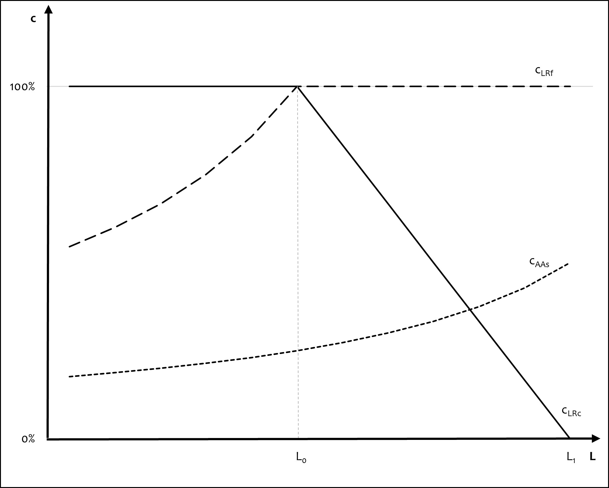
the land’s agricultural suitability is illustrated by the dotted line graph in Figure 2. The second coordinate of the points on the graphs presented in Figure 2 should be interpreted as the value of a given coefficient in relation to a unit,
homogenic agricultural plot (with area close to zero), included in a farm, which is
in the equilibrium point under the conditions of application of area support of a
given payment rate (E1), and thus involves L1 agricultural land inputs in the production process. The graph is illustrative; it
shows the development of the analysed variables at a given relation of the payment
rate to the production costs and revenue from the sale of the cultivated agricultural
product.
In Figure 1(b), the value of the subsidy coefficient for agricultural activities for a specific
homogeneous, one hectare land plot is the ratio of the vertical distance between the
MR0 line and the MR1 line (i.e., the area payment rate PR) to the vertical distance between the horizontal
axis and the MR1 line. Meanwhile, the value of this coefficient for a farm at equilibrium point E1 (i.e., using land input of size L1 for production) is the ratio of the area of parallelogram CBDE1 to the area of trapezoid COL1E1.
Within the proposed model, a theoretical decomposition of production factor remuneration
is made into income from non-land production factors and land rent. For the variant
with area payments, these two fractions of remuneration are further divided into part
financed by the market and part financed by the state. This allows for the introduction
of two additional indicators: the state co-financing coefficient of land rent and
the land rent-creation coefficient by area payments.
Based on Figure 1(b), it can be concluded that area support entirely contributes to land remuneration
in the case of land that was used for agricultural production even in the absence
of area payments (0<L≤L0). However, for land that was brought into production only after the introduction
of area payments at rate PR (L0<L≤L1), area support partly constitutes land remuneration and partly constitutes remuneration
for other production factors. It is worth noting that, as we move rightward along
the horizontal axis of the coordinate system from L0, an increasing portion of area support contributes to the remuneration of labour
and capital, while the portion allocated to land remuneration decreases. This means
that, as land productivity decreases, the market’s role in remunerating labour and
capital diminishes, while the state’s role increases. In the extreme case of the marginal
land plot L1, area support entirely contributes to labour and capital remuneration, while land
rent equals zero.
To measure what portion of land remuneration is financed by the state, we can introduce
the state co-financing coefficient of land rent (cLRf) expressed by the formula:
(2)
Where TC is the total cost, i.e. non-land production inputs, in relation to the land
area covered by area support, expressed in monetary units (m.u.).
Like the subsidy coefficient for agricultural activities, the state co-financing coefficient
of land rent is dimensionless and can take any value in the closed interval from 0
to 100%. Taking into account Figure 1(b), we can see that for the unit plot L0 and for plots located to the left of it, the state’s contribution to financing land
rent is expressed by the ratio of the area payment rate (PR) to the vertical distance
between the MC line and the MR1 line. This ratio increases as one moves rightward
along the horizontal axis. For plots located to the right of L0 (up to and including L1), the state’s contribution to financing land rent is 100% (since, in this case, both
the numerator and the denominator of the fraction expressing this contribution represent
the same number corresponding to the vertical distance between the MC and MR1 lines). However, this does not change the fact that, in absolute terms, land rent
decreases as one moves rightward along the horizontal axis of the coordinate system.
The dashed line graph in Figure 2 illustrates how the value of the state co-financing coefficient of land rent changes
depending on the agricultural suitability of the land. In relation to the entire farm
located at the equilibrium point E1, the state’s contribution to financing land rent is expressed as the ratio of the
area of trapezoid CBE0E1 to the area of triangle CAE1 (Figure 1(b)).
The land rent-creation coefficient by area payments (CLRc) indicates what portion of area support increases land rent. This indicator can be
expressed using the following formula:
(3)
Where ΔLR is the increase in land rent due to the introduction of area payments, expressed
in monetary units (m.u.).
Figure 2Values of the indicators measuring the impact of area payments on the distribution
sphere depending on the agricultural suitability of the land
Just like the indicators expressed by formulas (1) and (2), the land rent-creation coefficient by area payments is dimensionless, and the possible
values for this indicator range from 0% to 100%. Based on Figure 1(b), it can be concluded that for land that was used for agricultural production even
in the absence of area support (0 <L ≤ L0), the value of this coefficient is 100%. However, for land that was brought into
production only after the introduction of area payments at rate PR (L0 <L ≤ L1), this coefficient is less than 100% and decreases as one moves rightward along the
horizontal axis of the coordinate system (reaching zero for the unit plot L1). For example, for a homogeneous, one hectare unit plot LH, the land rent-creation coefficient equals the percentage ratio of the length of
segment |GH| to the length of segment |FH| (segment |FH| reflects the area payment
rate PR). Observing the continuous line graph in Figure 2, one can see how the value of this coefficient changes depending on the agricultural
suitability of the land. Meanwhile, the value of the land rent-creation coefficient
by area payments for all land included in the farm located at the equilibrium point
E1 can be calculated as the percentage ratio of the area of trapezoid CBE0E1 to the area of parallelogram CBDE1 (Figure 1(b)).
4.2.3. Implications for Lease Rent and Agricultural Land Prices
In cases where the user of the land is not its owner, land rent takes the form of
lease rent. As a result of area payments being at least partially transformed into
land rent, there is a phenomenon of “capturing” support by landowners through corresponding
increases in lease rent or land sale prices. In situations where land ownership is
separate from land use, the land rent-creation coefficient measures the extent to
which area payments are “captured” by landowners.
The “capture” of area support by agricultural landowners manifests itself in higher
lease rent rates and higher agricultural land prices, i.e., the capitalization of
payments. This occurs when the landowner is not identical to the land user, and when
the land is subject to market transactions. “Capturing” the payments involves factoring
part or all of the area support into the lease rent (in the case of leasing) or the
land price (in the case of selling), as a consequence of increased discounted income
from agricultural land due to the area payments.
The increase in the stream of discounted income from area payments (∆DISAP) can be calculated using the following formula:
(4)
Where CLRc is the land rent-creation coefficient by area payments (dimensionless); r is the
annual interest rate; and (n+1) is the number of years of area payment application.
The increase in lease rent for a given year following the introduction of area payments
corresponds to the increase in the annual income stream due to these payments, while
the entire increase in the stream of future discounted incomes will be capitalized
in the land price. Therefore, the first component of the sum in formula (4) represents the theoretical increase in lease rent in the first year of area payment
application, while the entire sum represents the theoretical increase in land price
in the event of a sale at the time the payments are introduced.
Calculating the future stream of income from area payments requires predicting payment
rates in subsequent years. In addition to issues related to predicting future income
streams from area support, various institutional conditions influence the process
of “capturing” area payments by agricultural landowners. In particular, the long-term
nature of lease agreements and their inflexibility result in inertia in lease rent
rates (), while legal restrictions on the agricultural land market may slow the process of
payment capitalization into land prices ().
4.3. Sensitivity analysis
A sensitivity analysis was carried out using illustrative numerical data. It allows
an assessment of the impact of the level of area support, measured by the payment
rate (PR), on selected variables, namely:
- Optimal land input (LE),
- The subsidy coefficient for agricultural activities (cAAs),
- The state co-financing coefficient of land rent (cLRf),
- The potential degree of “capture” of payments by landowners (by increasing lease
rents), which is the same as the land rent-creation coefficient by area payments (cLRc)
Table 2Level of area support and the value of key variables characterizing the production
sphere and the distribution sphere – sensitivity analysis using illustrative data
Area payment rate (PR)
Optimal land input (LE)
Subsidy coefficient for agricultural activities (cAAs)
State co-financing coefficient of land rent (cLRf)
Potential degree of payments “capture” by lessors (cLRc)
m.u./ha
ha
%
%
%
0
6
0,00%
0,00%
0,00%
0,25
7,5
6,25%
36,00%
90,00%
0,5
9
12,50%
55,56%
83,33%
0,75
10,5
18,75%
67,35%
78,57%
1
12
25,00%
75,00%
75,00%
1,25
13,5
31,25%
80,25%
72,22%
1,5
15
37,50%
84,00%
70,00%
Based on the results compiled in Table 2, it can be concluded that as the subsidy rate in the form of area payments increases:
The optimal land input increases (linearly), which means that farmers engage more
and more of the available agricultural land in the production process, even those
of lower quality or located more peripherally;
The share of the state in financing the remuneration of the factors of production
is increasing (linearly), which means that the state plays an increasing role in financing
agriculture, and thus the market efficiency of resource allocation is decreasing;
The share of the state in financing the remuneration of land as a factor of production
is increasing, with the rate of increase in the state’s role in financing land rents
falling faster than the rate of increase in the payment rate;
The potential degree of “capture” of payments by landowners through increases in rents
is declining, and the rate of decline in the degree of “capture” being less rapid
than the rate of increase in the payment rate.
5. CONCLUSIONS
The article presents an original model of the impact of area payments on the level
of engagement and remuneration of production factors in agriculture, including the
concept of three indicators measuring the scale of area payments’ impact on the distribution
sphere. Regarding the production sphere, the model allows for determining the optimal
land input on a farm. In terms of the distribution sphere, the model makes it possible
to establish the structure of non-market (i.e., state-funded) remuneration for production
factors into which area payments are converted. The practical usefulness of the model
lies in its ability to indicate the maximum lease rent level depending on the agricultural
suitability (productivity) of the land.
Based on the analysis conducted using the proposed model and a review of the relevant
literature, the following conclusions can be drawn:
1) Due to the direct support system, the production factors engaged in agriculture
generate remuneration that exceeds the monetary equivalent of the agricultural products
produced by farms. This additional remuneration, which goes beyond the monetary value
of the produced goods, is paid by the state in the form of direct payments, which
in the EU usually take the form of area payments.
2) The application of area payments promotes the inclusion of less fertile or peripherally
located land in cultivation, thus increasing the extensiveness of production.
3) The measure of relative support level is the subsidy coefficient for agricultural
activities, and its value increases as less agriculturally suitable land is brought
into production, because the lower the productivity of a plot of land, the greater
the portion of remuneration for production factors that comes from area support.
4) The state’s contribution to financing land rent increases as the agricultural suitability
of the land decreases. This contribution does not exceed 100% only for land that would
be cultivated even in the absence of area support.
5) Area support is wholly or partially transformed into land rent, and the measure
of this phenomenon is the land ent-creation coefficient. If the conversion of payments
into land rent is partial, besides supplementing land remuneration, they also co-finance
the input of other production factors, such as labour and capital. This occurs for
land that was brought into production as a result of the introduction of support.
6) Only for land that would be used for agricultural purposes even in the absence
of area payments is it possible to completely “capture” the area support by landowners
from land users.
7) If area support is reflected in the amount of lease rent, it indicates the presence
of the phenomenon of “capturing” area payments by landowners. This phenomenon also
manifests in land market transactions when the stream of discounted income from area
payments is capitalized into the price of land.
8) The “capturing” of area payments by landowners is countered, especially in the
early years of support applying, by the inertia of lease rates due to the inflexibility
of land lease agreements and the inertia of land prices caused by legal restrictions
on the agricultural land market.
9) Due to the direct link between the amount of payment and the area of agricultural
land used, area support is relatively susceptible to “capture” by landowners. Thus,
the effectiveness of this type of aid as an income support tool for farmers is therefore
greater the smaller the discrepancy between land ownership and land use.
In summary, the presented economic model demonstrates that area payments alter the
allocation of resources compared to the allocation driven by the market mechanism
(resulting in greater engagement of production factors in agricultural production
than would occur without these subsidies) and affect the size and structure of remuneration
for production factors in agriculture.
The added value of this study is manifested in three dimensions – cognitive, methodological,
and practical. Understanding the mechanism by which area payments stimulate the input
of production factors in agriculture and the mechanism through which subsidies granted
as area payments are converted into production factor remuneration is of cognitive
value. The model of area payment transformation into production factor remuneration
can serve as a basis for econometric modelling to predict the economic effects of
agricultural policy (ex-ante assessment) and to measure the effectiveness and efficiency
of agricultural policy instruments (ex-post assessment), which adds value in improving
research methodology. The knowledge gained from such studies facilitates the design
of agricultural policy tools and the adaptation of the instrumentation to changing
socio-economic conditions or revised political objectives, demonstrating the practical
potential of the presented model.
The proposed theoretical model may be particularly useful in a variant analysis of
alternative directions for agricultural policy reform, serving as a starting point
for an ex-ante assessment of the proposed changes. For instance, the model can be
used to identify the economic effects of the following adjustments in relation to
area-based support:
Changes in area payment rates – the model demonstrates how an increase or decrease
in these rates affects the engagement of production factors in agriculture and the
level of land rent;
Differentiation of payments based on land quality – the model allows for an assessment
of how adjusting support levels to land productivity could help mitigate the phenomenon
of subsidy “capture” by landowners;
Introduction of additional environmental conditions – indirectly, the model indicates
how linking payments to ecological practices could contribute to reducing the scale
of subsidy “capture” by landowners.
The model highlights the issue of payment capitalization in land prices and rental
rates. The essence of this problem is that a portion of the support – rather than
benefiting active farmers (land users) – instead increases the incomes of landowners,
making them the actual beneficiaries of agricultural policy. In this sense, the model
exposes the shortcomings of area payments as an instrument for supporting farmers'
incomes. The proposed model can facilitate the design of solutions that ensure more
effective targeting of area-based support, enhancing the efficiency of this instrument
in achieving its intended objectives.
Chatellier, V., & Guyomard. H. (2023). Supporting European farmers’ incomes through
Common Agricultural Policy direct aids: facts and questions. Review of Agricultural, Food and Environmental Studies, 104, 87–99. https://doi.org/10.1007/s41130-023-00192-8
3
Ciaian, P., & Kancs, d’A. (2012). The capitalization of area payments into farmland
rents: micro evidence from the new EU member states. Canadian Journal of Agricultural Economics, 60(4), 517–540. https://doi.org/10.1111/j.1744-7976.2012.01256.x
4
Ciaian, P., Baldoni, E., Kancs, d’A., & Drabik, D. (2021). The capitalization of agricultural
subsidies into land prices. Annual Review of Resource Economics, 13(1), 17–38. https://doi.org/10.1146/annurev-resource-102020-100625
5
Ciaian, P., Kancs, d'A., & Espinosa, M. (2018). The impact of the 2013 CAP reform
on the decoupled payments’ capitalisation into land values. Journal of Agricultural Economics, 69(2), 306–337. https://doi.org/10.1111/1477-9552.12253
6
Ciliberti, S., & Frascarelli, A. (2018). Does the basic payment efficiently enhance
farm incomes? Evidences from Italy. Paper presented at the 162nd European Association
of Agricultural Economists (EAAE) Seminar “The evaluation of new CAP instruments:
Lessons learned and the road ahead”, Budapest, Hungary, April 26–27, 2018. https://doi.org/10.22004/ag.econ.271957
7
Ciliberti, S., Palazzoni, L., Lilli, S.M., & Frascarelli. A., (2023). Direct payments
to provide environmental public goods and enhance farm incomes: do allocation criteria
matter? Review of Economics and Institutions, 13(1–2), 1–24. http://dx.doi.org/10.5281/zenodo.7604045
8
Czyżewski, A., & Poczta-Wajda, A. (2011). Polityka rolna w warunkach globalizacji. Doświadczenia GATT/WTO. Warszawa: Polskie Wydawnictwo Ekonomiczne.
9
Czyżewski, B., & Trojanek, R. (2016). Drivers of agricultural land prices in terms
of different functions of rural areas in Poland. Problems of Agricultural Economics, 347(2), 3–25. https://doi.org/10.30858/zer/83059
10
Czyżewski, B., Czyżewski, A., & Kryszak, Ł. (2019). The market treadmill against sustainable
income of European farmers: how the CAP has struggled with Cochrane’s curse. Sustainability, 11(3), 1–15. https://doi.org/10.3390/su11030791
11
De Castro, P., Miglietta P.P., & Vecchio, Y. (2020). The Common Agricultural Policy
2021–2027: a new history for European agriculture. Rivista Di Economia Agraria, 75(3), 5–12. https://doi.org/10.13128/rea-12703
12
Feichtinger, P., & Salhofer, K. (2013). What do we know about the influence of agricultural
support on agricultural land prices? German Journal of Agricultural Economics, 62(2), 71–85. https://doi.org/10.22004/ag.econ.232333
13
Feichtinger, P., & Salhofer, K. (2016). The Fischler Reform of the Common Agricultural
Policy and agricultural land prices. Land Economics, 92(3), 411–432. http://www.jstor.org/stable/24773491
14
Forstner, B., Duden, C., Ellßel, R., Gocht, A., Hansen, H., Neuenfeldt, S., Offermann,
F., & de Witte, T. (2018). Wirkungen von Direktzahlungen in der Landwirtschaft – ausgewählte
Aspekte mit Bezug zum Strukturwandel. Thünen Working Paper, 96. https://doi.org/10.3220/WP1524561399000
15
Gołasa, P., Bieńkowska-Gołasa, W., & Litwiniuk. P. (2023). The evolution of financial
instruments in the Common Agricultural Policy in light of the Strategic Plan for 2023–2027.
Studia Iuridica, 99, 346–361. https://doi.org/10.31338/2544-3135.si.2024-99.19
16
Góral, J., & Kulawik. J. (2015). Problem of capitalisation of subsidies in agriculture.
Problems of Agricultural Economics, 342(1), 3–23. https://doi.org/10.5604/00441600.1147600
17
Graubner, M. (2018). Lost in space? The effect of direct payments on land rental prices.
European Review of Agricultural Economics, 45(2), 143–171. https://doi.org/10.1093/erae/jbx027
18
Guastella, G., Moro, D., Sckokai, P., & Veneziani, M. (2021). The capitalisation of
decoupled payments in farmland rents among EU regions. Bio-Based and Applied Economics, 10(1), 7–17. https://doi.org/10.36253/bae-10034
19
Hennig, S., & Breustedt, G. (2018). The incidence of agricultural subsidies on rental
rates for grassland. Journal of Economics and Statistics, 238(2), 125–156. https://doi.org/10.1515/jbnst-2017-0124
20
Kilian, S., & Salhofer, K. (2008). Single payments of the CAP: where do the rents
go? Agricultural Economics Review, 9(2), 96–106. https://doi.org/10.22004/ag.econ.178238
21
Kilian, S., Antón, J., Salhofer, K., & Röder, N. (2012). Impacts of 2003 CAP Reform
on land rental prices and capitalization. Land Use Policy, 29(4), 789–797. https://doi.org/10.1016/j.landusepol.2011.12.004
22
Klaiber, H.A., Salhofer, K., & Thompson, S. (2017). Capitalisation of the SPS into
agricultural land rental prices under harmonisation of payments. Journal of Agricultural Economics, 68(3), 710–726. https://doi.org/10.1111/1477-9552.12207
23
Landreth, H., & Colander, D.C. (2001). History of economic thought, 5th ed. Boston: Houghton Mifflin.
24
Latruffe, L., & Le Mouël, C. (2009). Capitalization of government support in agricultural
land prices: What do we know? Journal of Economic Surveys, 23(4), 659–691. https://doi.org/10.1111/j.1467-6419.2009.00575.x
25
Majewski, E., Sulewski, P., & Wąs, A. (2018). Ewolucja Wspólnej Polityki Rolnej Unii Europejskiej w kontekście wyzwań trwałego rozwoju. Warszawa: Wydawnictwo Szkoły Głównej Gospodarstwa Wiejskiego.
26
Mata, F., Cano-Díaz, C., & Jesus, M. (2024). The European citizens’ stance on the
sustainability subsidies given to the EU farmers. European Countryside, 16(2), 324–336. https://doi.org/10.2478/euco-2024-0018
27
Michalek, J., Ciaian, P. & Kancs. d’A. (2014). Capitalization of the Single Payment
Scheme into land value: generalized propensity score evidence from the European Union.
Land Economics, 90(2), 260–289. http://www.jstor.org/stable/24243707
28
Morkunas, M., & Labukas, P. (2020). The evaluation of negative factors of direct payments
under Common Agricultural Policy from a viewpoint of sustainability of rural regions
of the new EU member states: Evidence from Lithuania. Agriculture, 10(6), 1–15. https://doi.org/10.3390/agriculture10060228
29
O’Neill, S., & Hanrahan, K. (2016). The capitalization of coupled and decoupled CAP
payments into land rental rates. Agricultural Economics, 47(3), 285–294. https://doi.org/10.1111/agec.12229
30
Patton, M., Kostov, P., McErlean, S., & Moss, J. (2008). Assessing the influence of
direct payments on the rental value of agricultural land. Food Policy, 33(5), 397–405. https://doi.org/10.1016/j.foodpol.2008.01.001
31
Pe'er, G., Bonn, A., Bruelheide, H., Dieker, P., Eisenhauer, N., Feindt, P.H., Hagedorn,
G., Hansjürgens, B., Herzon, I., Lomba, Â., Marquard, E., Moreira, F., Nitsch, H.,
Oppermann, R., Perino, A., Röder, N., Schleyer, C., Schindler, S., Wolf, C., Zinngrebe,
Y., & Lakner, S. (2020). Action needed for the EU Common Agricultural Policy to address
sustainability challenges. People and Nature, 2(2), 305–316. https://doi.org/10.1002/pan3.10080
32
Pilvere, I., Nipers, A., & Pilvere, A. (2022). Evaluation of the European Green Deal
Policy in the context of agricultural support payments in Latvia. Agriculture, 12(12), 1–22. https://doi.org/10.3390/agriculture12122028
33
Ricardo, D. (1996). Principles of political economy and taxation, 2nd ed. Amherst: Prometheus.
34
Sadłowski, A. (2012a). The reform of the Common Agricultural Policy after 2013 – adjusting
the instruments to the strategic plan for agriculture and rural development. Acta Scientiarum Polonorum. Oeconomia, 11(2), 57–66. https://aspe.sggw.edu.pl/article/view/567
35
Sadłowski, A. (2012b). Wpływ płatności bezpośrednich na warunki konkurencji na wspólnym
rynku europejskim. Wieś i Rolnictwo, 2(155), 82–96. https://doi.org/10.53098/wir.2012.2.155/05
36
Sadłowski, A. (2017). Impact of direct payments on the distribution area – model approach.
Problems of Agricultural Economics, 350(1), 75–100. https://doi.org/10.30858/zer/83000
Sadłowski, A. (2023). Decomposition of variations of direct payments rates on the
example of selected support instruments applied in Poland. Agricultural Economics, 69(2), 55–67. https://doi.org/10.17221/285/2022-AGRICECON
39
Sadłowski, A., Wrzaszcz, W., Smędzik-Ambroży, K., Matras-Bolibok, A., Budzyńska, A.,
Angowski, M., & Mann, S. (2021). Direct payments and sustainable agricultural development
– the example of Poland. Sustainability, 13(23), 1–20. https://doi.org/10.3390/su132313090
40
Salhofer, K., & Feichtinger, P. (2021). Regional differences in the capitalisation
of first and second pillar payments of the CAP into land rental prices. European Review of Agricultural Economics, 48(1), 8–41. https://doi.org/10.1093/erae/jbaa028
41
Scown, M.W., Brady, M.V., & Nicholas, K.A. (2020). Billions in misspent EU agricultural
subsidies could support the sustainable development goals. One Earth, 3(2), 237–250. https://doi.org/10.1016/j.oneear.2020.07.011
42
Stonkutė, E. (2009). Mapping the further developments of income support policy in
the EU. Management Theory and Studies for Rural Business and Infrastructure Development, 17(2), 105–113. https://www.lituanistika.lt/content/23677
43
Szerletics, Á., & Jámbor, A. (2020). The economic impacts of direct payments on agricultural
income – a literature review. Competitio, 19(1–2), 3–25. https://doi.org/10.21845/comp/2020/1-2/2
44
Van Herck, K., & Vranken, L. (2011). Direct payments and rent extraction by land owners:
Evidence from new member states. Paper presented at the 122nd European Association
of Agricultural Economists (EAAE) “Evidence-based agricultural and rural policy making:
methodological and empirical challenges of policy evaluation” Seminar, Ancona, Italy,
February 17–18, 2011. https://doi.org/10.22004/ag.econ.99583
45
Van Tongeren, F. (2008). Agricultural Policy Design and Implementation: A Synthesis.
OECD Food, Agriculture and Fisheries Papers, 7, 1–31. http://dx.doi.org/10.1787/243786286663
46
Varacca, A., Guastella, G., Pareglio, S., & Sckokai, P. (2022). A meta-analysis of
the capitalisation of CAP direct payments into land prices. European Review of Agricultural Economics, 49(2), 359–382. https://doi.org/10.1093/erae/jbab014
[1] In the EU Member States applying the SPS, the stimulating effect of area payments
on the overall level of land use in agriculture was prevented by establishing an area
limit on a national scale as a resultant of the total (fixed) number of payment entitlements.